Conditional Formatting with Nested IF Function in Excel

[Admin]

To meet multiple conditions in data or record, Excel offers the nested if function. We know, the IF function has three arguments – in case of nesting, you can replace one of the arguments with another function – it can be another IF function or SUM function or AVERAGE function and so on. It depends on the reqiurements of how you want to assess your data.


In the following table, I want to classify or assess my data as follows: if the temperature is

below - 8°C, then „Hard Winter“,

0 to - 8°C as „Cold“,

0 to 5°C as „Mild“,

5 to 12°C as „Good“, and

above 12°C as „Warm“.



So in cell C2 enter

=IF(B2<=-8;"Hard Winter";IF(B2<=0;"Cold";IF(B2<=5;"Mild";IF(AND(B2>5;B2<=12);"Good";"Warm"))))





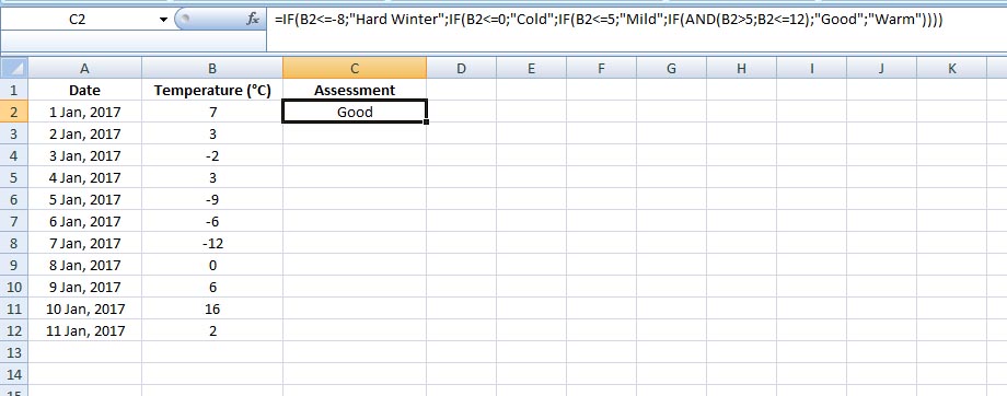
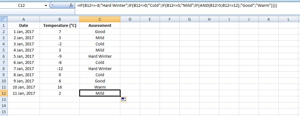
Now copy it down the column.







Now do the conditional formatting


In Excel, you can highlight cell values with colors through conditional formatting, to quickly capture important information in your spreadsheet. We will do it here step-by-step to highlight our data based on their values:

Select the range (C2:C12)

Click on Conditional Formatting (you find it under the Home Tab) > Click on New Rule...






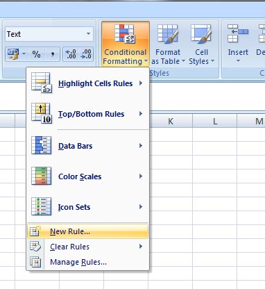
The New Formatting Rule window opens.

from Select a Rule Type > click on Format only cells that contain

here under Format only cells with > select Specific Text > type Hard Winter in the empty box

from the Format... below > select Red color > Click OK.





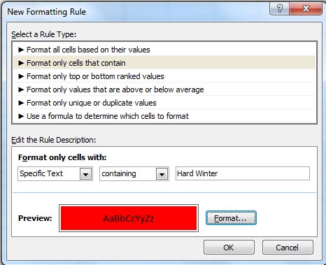
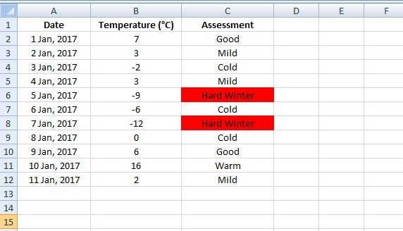
Now you will see that in Column C cells containing Hard Winter are marked with red.






Go ahead for the rest:

Select your range again (C2:C12) > click on Conditional Formatting > this time click on Manage Rules...

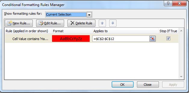
The Conditional Formatting Rules Manager window opens. Here you can see the first condition you just specified for Hard Winter.






Click on New Rule... > the New Formatting Rule window opens. Do like before:

from Select a Rule Type > click on Format only cells that contain

here under Format only cells with > select Specific Text > type Cold in the empty box

from the Format... below > select any color of your choice > click OK.


Repeat the same procedure from the Conditional Formatting Rules Manager dialog box : I mean, click again on New Rule..... and so on ….... you move on > click on OK.






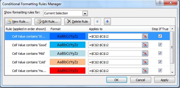
If you want to edit the colors or other options, either double click on any colorband or click on Edit Rule..., the Edit Formatting Rule window will open.


You can always do editing anytime later.

Just select your range > go to Conditional Formatting > click on Manage Rules...


By the way your temperature table has now a new look & feel






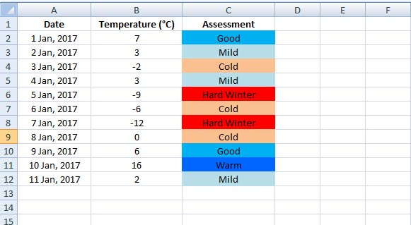
Do experiment with conditional formatting – it's fun and makes you easy-going with one of Excel's most useful tools.

Have fun




*You may also need to read:

How to use 'IF Function' in Excel – written in a very easy way





*Recommended:

Read wonderful articles (English & German) on Science & Tech, Environment, Health and many other topics only on BlogArena.

For comments of suggestions, please contact us: info@shamskm.com